首页 › 网站首页 ›商业资讯› 数据 › 查看内容

实例 | 分析38万条数据，分析保险行业中的数据应用

私域流量数据 2022-12-8 11:55 8396人围观

CDA数据分析师出品编辑：Mika

明天的内容是一期Python实战练习，我们来手把手教你用Python分析保险产物穿插销售和哪些身分有关。

01实战布景

首先先容下实战的布景：

此次的数据集来自kaggle：

https://www.kaggle.com/anmolkumar/health-insurance-cross-sell-prediction

我们的客户是一家保险公司，比来新推出了一款汽车保险。现在他们的需如果建立一个模子，用来猜测客岁的投保人能否会对这款汽车保险感爱好。

我们晓得，保险单指的是，保险公司许诺为特定范例的损失、侵害、疾病或灭亡供给补偿保证，客户则需要定期向保险公司付出一定的保险费。

这里再进一步说明一下。

例如，你每年要为20万的健康保险付出2000元的保险费。那末你必定会想，保险公司只收取5000元的保费，这类情况下，怎样能承当如此高的住院用度呢? 这时，“几率”的概念就出现了。例如，像你一样，能够有100名客户每年付出2000元的保费，但昔时住院的能够只要少数人，(比如2-3人)，而不是一切人。经过这类方式，每小我都分管了其他人的风险。

和医疗保险一样，买了车险的话，每年都需要向保险公司付出一定数额的保险费，这样在车辆发买卖外变乱时，保险公司将向客户供给补偿（称为“保险金额”）。

我们要做的就是建立模子，来猜测客户能否对汽车保险感爱好。这对保险公司来说是很是有帮助的，公司可以据此制定相同战略，打仗这些客户，并优化其贸易形式和支出。

02数据了解

为了猜测客户能否对车辆保险感爱好，我们需方法会一些客户信息 (性别、年龄等)、车辆(车龄、损坏情况)、保单(保费、采购渠道)等信息。

数据分别为练习集和测试集，练习数据包括381109笔客户材料，每笔客户材料包括12个字段，1个客户ID字段、10个输入字段及1个方针字段-Response能否响应(1代表感爱好，0代表不感爱好)。测试数据包括127037笔客户材料；字段个数与练习数据不异，方针字段没有值。字段的界说可参考下文。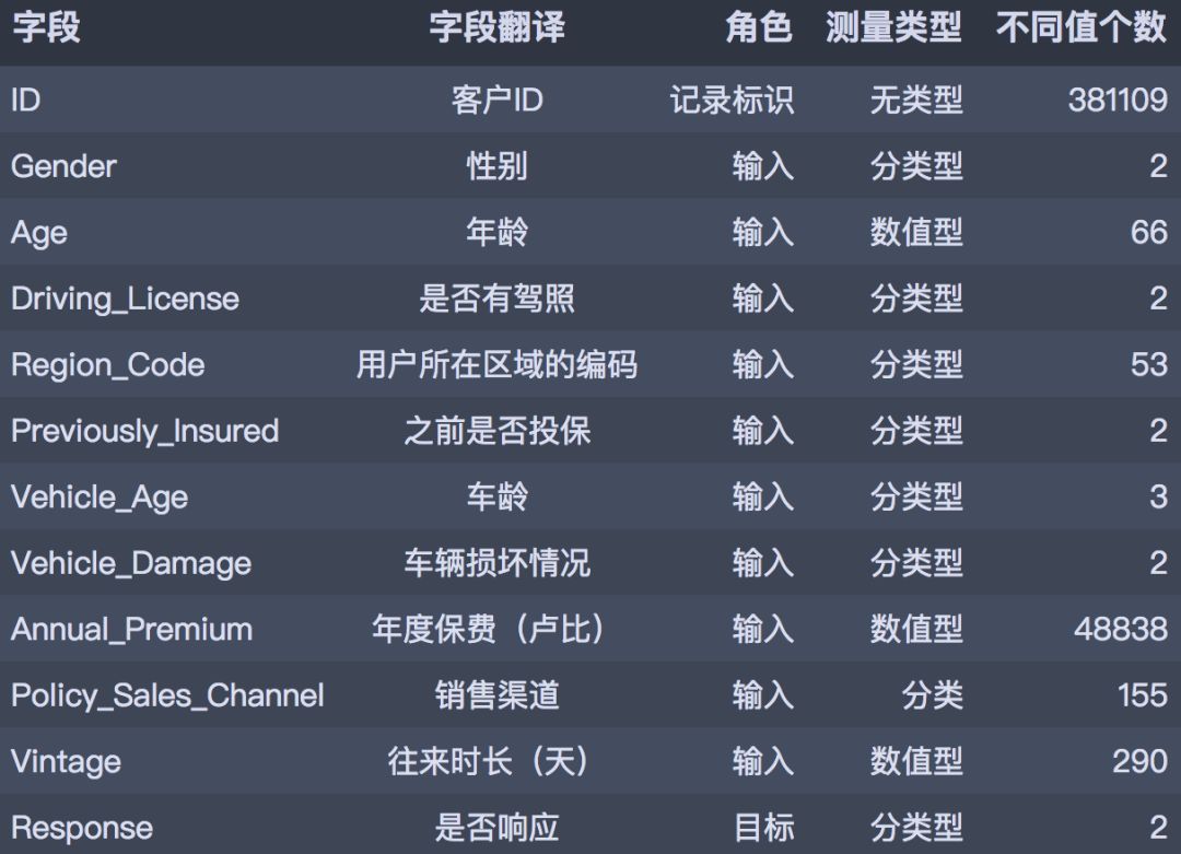

下面我们起头吧！

03数据读入和预览

首先起头数据读入和预览。

# 数据整理
import numpy as np
import pandas as pd

# 可视化
import matplotlib.pyplot as plt
import seaborn as sns
import plotly as py
import plotly.graph_objs as go
import plotly.express as px
pyplot = py.offline.plot
from exploratory_data_analysis import EDAnalysis # 自界说# 读入练习集
train = pd.read_csv('../data/train.csv')
train.head()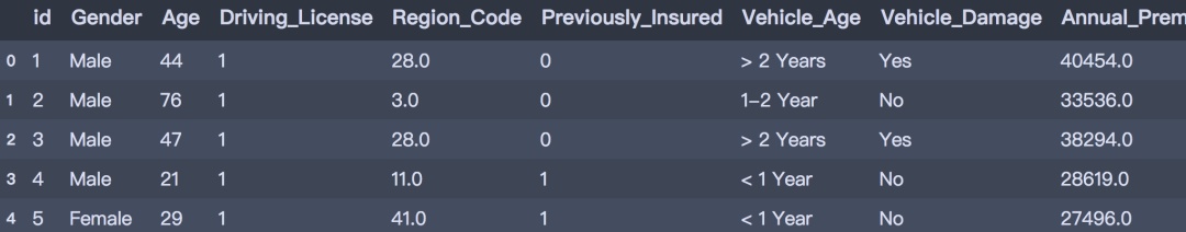

# 读入测试集
test = pd.read_csv('../data/test.csv')
test.head()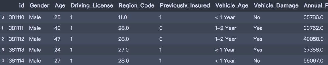

print(train.info())
print('-' * 50)
print(test.info()) <class 'pandas.core.frame.DataFrame'>
RangeIndex: 381109 entries, 0 to 381108
Data columns (total 12 columns):
# Column Non-Null Count Dtype
--- ------ -------------- -----
0 id 381109 non-null int64
1 Gender 381109 non-null object
2 Age 381109 non-null int64
3 Driving_License 381109 non-null int64
4 Region_Code 381109 non-null float64
5 Previously_Insured 381109 non-null int64
6 Vehicle_Age 381109 non-null object
7 Vehicle_Damage 381109 non-null object
8 Annual_Premium 381109 non-null float64
9 Policy_Sales_Channel 381109 non-null float64
10 Vintage 381109 non-null int64
11 Response 381109 non-null int64
dtypes: float64(3), int64(6), object(3)
memory usage: 34.9+ MB
None
--------------------------------------------------
<class 'pandas.core.frame.DataFrame'>
RangeIndex: 127037 entries, 0 to 127036
Data columns (total 11 columns):
# Column Non-Null Count Dtype
--- ------ -------------- -----
0 id 127037 non-null int64
1 Gender 127037 non-null object
2 Age 127037 non-null int64
3 Driving_License 127037 non-null int64
4 Region_Code 127037 non-null float64
5 Previously_Insured 127037 non-null int64
6 Vehicle_Age 127037 non-null object
7 Vehicle_Damage 127037 non-null object
8 Annual_Premium 127037 non-null float64
9 Policy_Sales_Channel 127037 non-null float64
10 Vintage 127037 non-null int64
dtypes: float64(3), int64(5), object(3)
memory usage: 10.7+ MB
None

04摸干脆分析

下面，我们基于练习数据集停止摸干脆数据分析。

1. 描写性分析

首先对数据集合数值型属性停止描写性统计分析。

desc_table = train.drop(['id', 'Vehicle_Age'], axis=1).describe().T
desc_table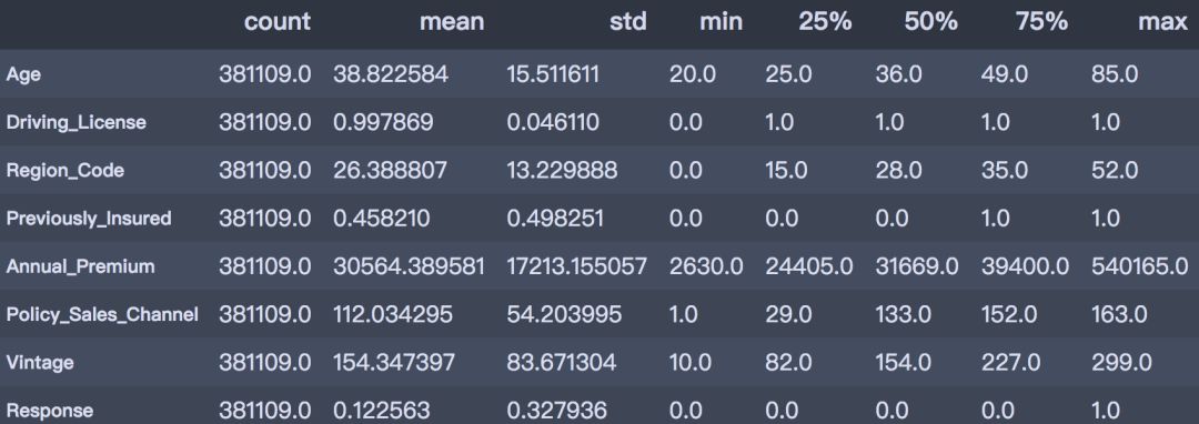

经过描写性分析后，可以获得以下结论。

从以上描写性分析成果可以得出：

客户年龄：客户的年龄范围在20 ~ 85岁之间，均匀年龄是38岁，青年群体居多；
能否有驾照：99.89%客户都持有驾照；
之前能否投保：45.82%的客户已经采办了车辆保险；
年度保费：客户的保费范围在2630 ~ 540165之间，均匀的保费金额是30564。
来往时长：此数据基于曩昔一年的数据，客户的来往时候范围在10~299天之间，均匀来往时长为154天。
能否响应：均匀来看，客户对车辆保险感爱好的几率为12.25%。

2. 方针变量的散布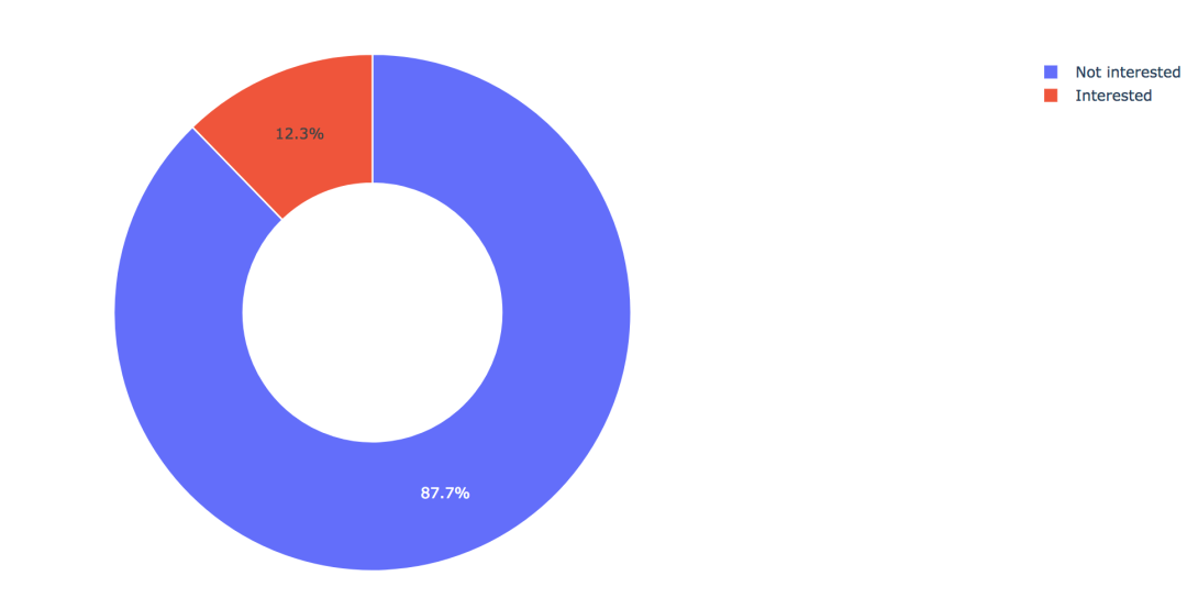

练习集共有381109笔客户材料，其中感爱好的有46710人，占比12.3%，不感爱好的有334399人，占比87.7%。

train['Response'].value_counts()
0 334399
1 46710
Name: Response, dtype: int64values = train['Response'].value_counts().values.tolist()

# 轨迹
trace1 = go.Pie(labels=['Not interested', 'Interested'],
values=values,
hole=.5,
marker={'line': {'color': 'white', 'width': 1.3}}
)
# 轨迹列表
data = [trace1]
# 结构
layout = go.Layout(title=f'Distribution_ratio of Response', height=600)
# 画布
fig = go.Figure(data=data, layout=layout)
# 天生HTML
pyplot(fig, filename='./html/方针变量散布.html')

3. 性别身分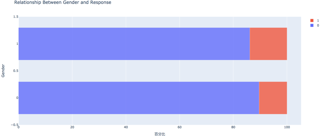

从条形图可以看出，男性的客户群体对汽车保险感爱好的几率稍高，是13.84%，相较女性客户横跨3个百分点。

pd.crosstab(train['Gender'], train['Response'])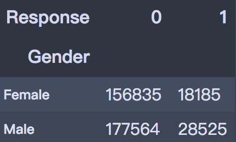

# 实例类
eda = EDAnalysis(data=train, id_col='id', target='Response')

# 柱形图
fig = eda.draw_bar_stack_cat(colname='Gender')
pyplot(fig, filename='./html/性别与能否感爱好.html')

4. 之前能否投保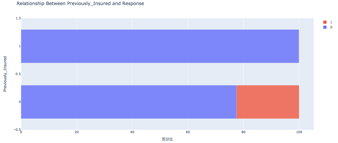

没有采办汽车保险的客户响应几率更高，为22.54%，有采办汽车保险的客户则没有这一需求，感爱好的几率仅为0.09%。

pd.crosstab(train['Previously_Insured'], train['Response'])

fig = eda.draw_bar_stack_cat(colname='Previously_Insured')
pyplot(fig, filename='./html/之前能否投保与能否感爱好.html')

5. 车龄身分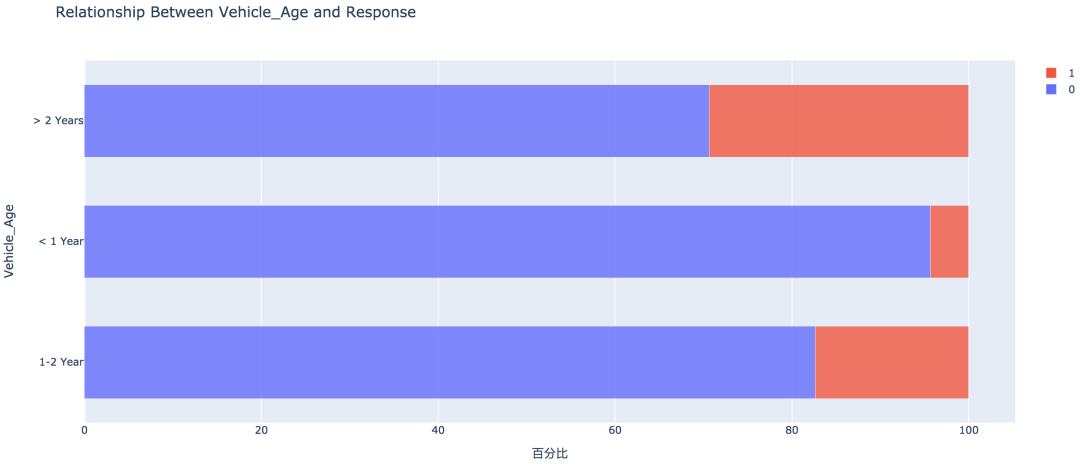

车龄越大，响应几率越高，大于两年的车龄感爱好的几率最高，为29.37%，其次是1~2年车龄，几率为17.38%。小于1年的仅为4.37%。

6. 车辆损坏情况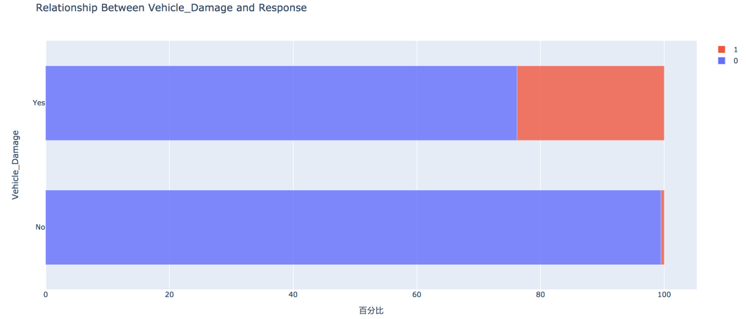

车辆已经损坏过的客户有较高的响应几率，为23.76%，相比之下，客户曩昔车辆没有损坏的响应几率仅为0.52%

7. 分歧年龄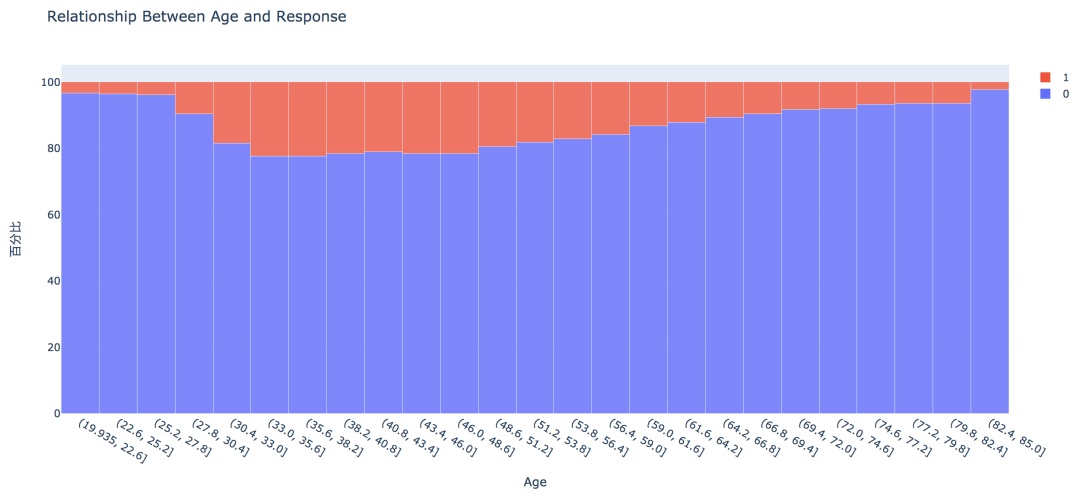

从直方图中可以看出，年龄较高的群体和较低的群体响应的几率较低，30~60岁之前的客户响应几率较高。

经过可视化摸索，我们大致可以晓得:

车龄在1年以上，之前有车辆损坏的情况出现，且未采办过车辆保险的客户有较高的响应几率。

05数据预处置

此部合作作首要包括字段挑选，数据清洗和数据编码，字段的处置以下：

Region_Code和Policy_Sales_Channel：分类数过量，且不易解读，删除；
Annual_Premium：异常值处置
Gender、Vehicle_Age、Vehicle_Damage：分范例数据转换为数值型编码

# 删除字段
train = train.drop(['Region_Code', 'Policy_Sales_Channel'], axis=1)

# 盖帽法处置异常值
f_max = train['Annual_Premium'].mean() + 3*train['Annual_Premium'].std()
f_min = train['Annual_Premium'].mean() - 3*train['Annual_Premium'].std()

train.loc[train['Annual_Premium'] > f_max, 'Annual_Premium'] = f_max
train.loc[train['Annual_Premium'] < f_min, 'Annual_Premium'] = f_min

# 数据编码
train['Gender'] = train['Gender'].map({'Male': 1, 'Female': 0})
train['Vehicle_Damage'] = train['Vehicle_Damage'].map({'Yes': 1, 'No': 0})
train['Vehicle_Age'] = train['Vehicle_Age'].map({'< 1 Year': 0, '1-2 Year': 1, '> 2 Years': 2})
train.head()

测试集做不异的处置：

# 删除字段
test = test.drop(['Region_Code', 'Policy_Sales_Channel'], axis=1)
# 盖帽法处置
test.loc[test['Annual_Premium'] > f_max, 'Annual_Premium'] = f_max
test.loc[test['Annual_Premium'] < f_min, 'Annual_Premium'] = f_min

# 数据编码
test['Gender'] = test['Gender'].map({'Male': 1, 'Female': 0})
test['Vehicle_Damage'] = test['Vehicle_Damage'].map({'Yes': 1, 'No': 0})
test['Vehicle_Age'] = test['Vehicle_Age'].map({'< 1 Year': 0, '1-2 Year': 1, '> 2 Years': 2})
test.head()

06数据建模

我们挑选利用以下几种模子停止建置，并比力模子的分类效能。

首先在将练习集分别为练习集和考证集，其中练习集用于练习模子，考证集用于考证模子结果。首先导入建模库：

# 建模
from sklearn.linear_model import LogisticRegression
from sklearn.neighbors import KNeighborsClassifier
from sklearn.tree import DecisionTreeClassifier
from sklearn.ensemble import RandomForestClassifier
from lightgbm import LGBMClassifier

# 预处置
from sklearn.preprocessing import StandardScaler, MinMaxScaler

# 模子评价
from sklearn.model_selection import train_test_split, GridSearchCV
from sklearn.metrics import confusion_matrix, classification_report, accuracy_score, f1_score, roc_auc_score# 分别特征和标签
X = train.drop(['id', 'Response'], axis=1)
y = train['Response']

# 分别练习集和考证集(分层抽样)
X_train, X_val, y_train, y_val = train_test_split(X, y, test_size=0.2, stratify=y, random_state=0)
print(X_train.shape, X_val.shape, y_train.shape, y_val.shape)
(304887, 8) (76222, 8) (304887,) (76222,)# 处置样本不服衡，对0类样本停止降采样
from imblearn.under_sampling import RandomUnderSampler

under_model = RandomUnderSampler(sampling_strategy={0:133759, 1:37368}, random_state=0)
X_train, y_train = under_model.fit_sample(X_train, y_train)
# 保存一份极值标准化的数据
mms = MinMaxScaler()

X_train_scaled = pd.DataFrame(mms.fit_transform(X_train), columns=x_under.columns)
X_val_scaled = pd.DataFrame(mms.transform(X_val), columns=x_under.columns)

# 测试集
X_test = test.drop('id', axis=1)
X_test_scaled = pd.DataFrame(mms.transform(X_test), columns=X_test.columns)

1. KNN算法

# 建立knn
knn = KNeighborsClassifier(n_neighbors=3, n_jobs=-1)
knn.fit(X_train_scaled, y_train)

y_pred = knn.predict(X_val_scaled)

print('Simple KNeighborsClassifier accuracy：%.3f' % (accuracy_score(y_val, y_pred)))
print('Simple KNeighborsClassifier f1_score: %.3f' % (f1_score(y_val, y_pred)))
print('Simple KNeighborsClassifier roc_auc_score: %.3f' % (roc_auc_score(y_val, y_pred))) Simple KNeighborsClassifier accuracy：0.807
Simple KNeighborsClassifier f1_score: 0.337
Simple KNeighborsClassifier roc_auc_score: 0.632# 对测试集评价
test_y = knn.predict(X_test_scaled)
test_y[:5]
array([0, 0, 1, 0, 0], dtype=int64)

2. Logistic回归

# Logistic回归
lr = LogisticRegression()
lr.fit(X_train_scaled, y_train)

y_pred = lr.predict(X_val_scaled)

print('Simple LogisticRegression accuracy：%.3f' % (accuracy_score(y_val, y_pred)))
print('Simple LogisticRegression f1_score: %.3f' % (f1_score(y_val, y_pred)))
print('Simple LogisticRegression roc_auc_score: %.3f' % (roc_auc_score(y_val, y_pred)))Simple LogisticRegression accuracy：0.863
Simple LogisticRegression f1_score: 0.156
Simple LogisticRegression roc_auc_score: 0.536

3. 决议树

# 决议树
dtc = DecisionTreeClassifier(max_depth=10, random_state=0)
dtc.fit(X_train, y_train)

y_pred = dtc.predict(X_val)

print('Simple DecisionTreeClassifier accuracy：%.3f' % (accuracy_score(y_val, y_pred)))
print('Simple DecisionTreeClassifier f1_score: %.3f' % (f1_score(y_val, y_pred)))
print('Simple DecisionTreeClassifier roc_auc_score: %.3f' % (roc_auc_score(y_val, y_pred))) Simple DecisionTreeClassifier accuracy：0.849
Simple DecisionTreeClassifier f1_score: 0.310
Simple DecisionTreeClassifier roc_auc_score: 0.603

4. 随机森林

# 决议树
rfc = RandomForestClassifier(n_estimators=100, max_depth=10, n_jobs=-1)
rfc.fit(X_train, y_train)

y_pred = rfc.predict(X_val)

print('Simple RandomForestClassifier accuracy：%.3f' % (accuracy_score(y_val, y_pred)))
print('Simple RandomForestClassifier f1_score: %.3f' % (f1_score(y_val, y_pred)))
print('Simple RandomForestClassifier roc_auc_score: %.3f' % (roc_auc_score(y_val, y_pred))) Simple RandomForestClassifier accuracy：0.870
Simple RandomForestClassifier f1_score: 0.177
Simple RandomForestClassifier roc_auc_score: 0.545

5. LightGBM

lgbm = LGBMClassifier(n_estimators=100, random_state=0)
lgbm.fit(X_train, y_train)

y_pred = lgbm.predict(X_val)

print('Simple LGBM accuracy: %.3f' % (accuracy_score(y_val, y_pred)))
print('Simple LGBM f1_score: %.3f' % (f1_score(y_val, y_pred)))
print('Simple LGBM roc_auc_score: %.3f' % (roc_auc_score(y_val, y_pred))) Simple LGBM accuracy: 0.857
Simple LGBM f1_score: 0.290
Simple LGBM roc_auc_score: 0.591

综上，以f1-score作为评价标准的情况下，KNN算法有较好的分类效能，这能够是由于数据样本自己不服衡致使，后续可以经过其他种别不服衡的方式做进一步处置，同时可以经过参数调剂的方式来优化其他模子，经过调剂猜测的门坎值来增加猜测效能等其他方式。